毒蘑菇的二元预测

您提供了很多关于不同二元分类任务的资源和链接，看起来这些都是Kaggle竞赛中的参考资料和高分解决方案。为了帮助您更好地利用这些资源，这里是一些关键点的总结：

Playground Season 4 Episode 8

• 主要关注的竞赛: 使用银行流失数据集进行二元分类。
• 数据集: 已经重新组织并发布供参考。
• 热门解决方案:

• • LightGBM 和 CatBoost 模型 (得分 0.8945)。
  • XGBoost 和随机森林模型。
  • 神经网络分类模型。

其他相关的竞赛和资源

• 使用生物信号对吸烟者状况进行二元预测

• • EDA 和特征工程。
  • XGBoost 模型。

• 使用软件缺陷数据集进行二元分类

• • EDA 和建模。

• 机器故障的二元分类

• • EDA, 集成学习, ML pipeline, SHAP 分析。

• 使用表格肾结石预测数据集进行二元分类

• • 多种模型对比。

• 特色竞赛

• • 美国运通 - 违约预测

• • • 特征工程和LightGBM模型。

• • 房屋信贷违约风险

• • • 完整的EDA和特征重要性分析。

竞争指标 - Mathews 相关性系数

• 定义: 衡量二元分类器输出质量的度量。
• 资源:

• • Wikipedia 关于 Phi 系数的页面。
  • Voxco 博客关于 Matthews 相关性系数的文章。
  • 一篇关于 Matthews 相关性系数在生物数据挖掘中的应用的论文。
  • Scikit-learn 文档中关于 Matthews 相关性系数的说明。

希望这些信息能够帮助您更有效地开始学习和参与这些竞赛。如果您有具体的问题或者需要针对某个特定部分的帮助，请告诉我！

# 加载训练数据
train_data = pd.read_csv('train.csv')# 显示前几行数据以了解数据结构
print(train_data.head())# 查看数据的基本信息
print(train_data.info())

步骤 2: 数据探索与可视化

在这一步中，我们将对数据进行更深入的探索，并使用可视化工具来更好地理解数据的分布和特征之间的关系。

# 统计每种类型的蘑菇数量
print(train_data['class'].value_counts())# 可视化不同类型的蘑菇数量
plt.figure(figsize=(8, 6))
sns.countplot(x='class', data=train_data)
plt.title('Distribution of Mushroom Classes')
plt.show()# 查看各特征与目标变量之间的关系
fig, axs = plt.subplots(5, 5, figsize=(20, 20))
axs = axs.flatten()
for i, col in enumerate(train_data.columns[1:]):sns.countplot(x=col, hue='class', data=train_data, ax=axs[i])axs[i].set_title(f'Distribution of {col} by Class')
plt.tight_layout()
plt.show()

步骤 3: 数据预处理

接下来，我们将对数据进行预处理，包括特征编码和其他必要的变换。

# 对类别特征进行编码
label_encoder = LabelEncoder()# 遍历所有非数字特征
for col in train_data.select_dtypes(include=['object']).columns:train_data[col] = label_encoder.fit_transform(train_data[col])# 查看编码后的数据
print(train_data.head())

步骤 4: 构建模型

在这一步中，我们将构建 LightGBM 和 CatBoost 模型，并进行训练。

# 分割数据集
X = train_data.drop('class', axis=1)
y = train_data['class']# 划分训练集和验证集
X_train, X_val, y_train, y_val = train_test_split(X, y, test_size=0.2, random_state=42)# 定义 LightGBM 模型
lgb_params = {'objective': 'binary','metric': 'auc','verbosity': -1,'boosting_type': 'gbdt','num_leaves': 31,'learning_rate': 0.05,'feature_fraction': 0.9,'bagging_fraction': 0.8,'bagging_freq': 5,'lambda_l1': 0.1,'lambda_l2': 0.1
}# 创建 LightGBM 数据集
lgb_train = lgb.Dataset(X_train, y_train)
lgb_val = lgb.Dataset(X_val, y_val, reference=lgb_train)# 训练 LightGBM 模型
lgb_model = lgb.train(lgb_params, lgb_train, num_boost_round=1000, valid_sets=[lgb_val], early_stopping_rounds=100)# 定义 CatBoost 模型
cb_params = {'loss_function': 'Logloss','eval_metric': 'AUC','learning_rate': 0.05,'depth': 6,'l2_leaf_reg': 10,'bootstrap_type': 'Bayesian','bagging_temperature': 0.2,'random_seed': 42,'allow_writing_files': False
}# 创建 CatBoost 数据集
cb_train = Pool(X_train, y_train)
cb_val = Pool(X_val, y_val)# 训练 CatBoost 模型
cb_model = CatBoostClassifier(**cb_params)
cb_model.fit(X_train, y_train, eval_set=(X_val, y_val), use_best_model=True, verbose=False)

步骤 5: 测试数据预测

最后，我们将使用训练好的模型对测试数据进行预测，并整理预测结果以符合 Kaggle 提交的要求。

# 加载测试数据
test_data = pd.read_csv('test.csv')# 对测试数据进行相同的特征编码
for col in test_data.select_dtypes(include=['object']).columns:test_data[col] = label_encoder.transform(test_data[col])# 获取测试数据的 ID
test_ids = test_data['id']# 删除不需要的列
test_features = test_data.drop('id', axis=1)# 使用模型进行预测
predictions_lgb = lgb_model.predict(test_features, num_iteration=lgb_model.best_iteration)
predictions_cb = cb_model.predict(test_features)# 将预测结果转换为二进制形式
predictions_lgb_binary = (predictions_lgb > 0.5).astype(int)
predictions_cb_binary = (predictions_cb > 0.5).astype(int)# 整理预测结果
submission_df = pd.DataFrame({'id': test_ids, 'class': predictions_lgb_binary})
submission_df['class'] = submission_df['class'].map({1: 'p', 0: 'e'})# 保存预测结果
submission_df.to_csv('submission.csv', index=False)

好的，现在我将为你提供一个完整的代码示例来解决“毒蘑菇的二元预测”问题。我们将使用 LightGBM 和 CatBoost 这两个模型来进行预测，并遵循之前讨论过的步骤。

首先，我们需要安装必要的库。如果你还没有安装它们，可以使用以下命令安装：

pip install pandas numpy scikit-learn lightgbm catboost matplotlib seaborn plotly

下面是完整的代码示例：

import pandas as pd
import numpy as np
import matplotlib.pyplot as plt
import seaborn as sns
import plotly.express as px
from plotly.subplots import make_subplots
import plotly.graph_objects as go
from sklearn.preprocessing import LabelEncoder
from sklearn.model_selection import train_test_split
import lightgbm as lgb
from catboost import CatBoostClassifier
from sklearn.metrics import matthews_corrcoef# 忽略警告
import warnings
warnings.filterwarnings('ignore')# 加载数据
train_data = pd.read_csv('train.csv')
test_data = pd.read_csv('test.csv')# 数据预处理
def preprocess_data(data):# 对类别特征进行编码label_encoder = LabelEncoder()for col in data.select_dtypes(include=['object']).columns:data[col] = label_encoder.fit_transform(data[col])return data# 预处理训练数据
train_data = preprocess_data(train_data)# 预处理测试数据
test_data = preprocess_data(test_data)# 数据分割
X = train_data.drop('class', axis=1)
y = train_data['class']
X_train, X_val, y_train, y_val = train_test_split(X, y, test_size=0.2, random_state=42)# 定义 LightGBM 模型
lgb_params = {'objective': 'binary','metric': 'binary_logloss','verbosity': -1,'boosting_type': 'gbdt','num_leaves': 31,'learning_rate': 0.05,'feature_fraction': 0.9,'bagging_fraction': 0.8,'bagging_freq': 5,'lambda_l1': 0.1,'lambda_l2': 0.1
}# 创建 LightGBM 数据集
lgb_train = lgb.Dataset(X_train, y_train)
lgb_val = lgb.Dataset(X_val, y_val, reference=lgb_train)# 训练 LightGBM 模型
lgb_model = lgb.train(lgb_params, lgb_train, num_boost_round=1000, valid_sets=[lgb_val], early_stopping_rounds=100)# 定义 CatBoost 模型
cb_params = {'loss_function': 'Logloss','eval_metric': 'AUC','learning_rate': 0.05,'depth': 6,'l2_leaf_reg': 10,'bootstrap_type': 'Bayesian','bagging_temperature': 0.2,'random_seed': 42,'allow_writing_files': False
}# 训练 CatBoost 模型
cb_model = CatBoostClassifier(**cb_params)
cb_model.fit(X_train, y_train, eval_set=(X_val, y_val), use_best_model=True, verbose=False)# 测试数据预测
test_ids = test_data['id']
test_features = test_data.drop('id', axis=1)# 使用 LightGBM 进行预测
predictions_lgb = lgb_model.predict(test_features, num_iteration=lgb_model.best_iteration)
predictions_lgb_binary = (predictions_lgb > 0.5).astype(int)# 使用 CatBoost 进行预测
predictions_cb = cb_model.predict(test_features)
predictions_cb_binary = (predictions_cb > 0.5).astype(int)# 评估模型
mcc_lgb = matthews_corrcoef(y_val, lgb_model.predict(X_val, num_iteration=lgb_model.best_iteration) > 0.5)
mcc_cb = matthews_corrcoef(y_val, cb_model.predict(X_val) > 0.5)print("LightGBM Matthews Correlation Coefficient: ", mcc_lgb)
print("CatBoost Matthews Correlation Coefficient: ", mcc_cb)# 整理预测结果
submission_df = pd.DataFrame({'id': test_ids, 'class': predictions_lgb_binary})
submission_df['class'] = submission_df['class'].map({1: 'p', 0: 'e'})# 保存预测结果
submission_df.to_csv('submission.csv', index=False)# 可视化特征重要性
def plot_feature_importance(model, feature_names, title):fig, ax = plt.subplots(figsize=(12, 8))lgb.plot_importance(model, max_num_features=20, importance_type='gain', ax=ax)ax.set_title(title)plt.show()# 可视化 LightGBM 特征重要性
plot_feature_importance(lgb_model, X_train.columns, 'LightGBM Feature Importance')# 可视化 CatBoost 特征重要性
cb_model.plot_feature_importances(top_n=20, figsize=(12, 8), title='CatBoost Feature Importance')

这段代码完成了以下任务：

1. 导入所需的库。
2. 加载训练数据和测试数据。
3. 对数据进行预处理，包括对类别特征进行编码。
4. 划分数据集为训练集和验证集。
5. 定义并训练 LightGBM 和 CatBoost 模型。
6. 对测试数据进行预测。
7. 评估模型的性能（使用 Matthews Correlation Coefficient）。
8. 整理预测结果，并将其保存为 CSV 文件以供提交。
9. 可视化特征重要性。

参考

Binary Classification with a Bank Churn Dataset

Playground Series - Season 4, Episode 1

OverviewDataCodeModelsDiscussionLeaderboardRulesTeamSubmissions

Samvel Kocharyan · 17th in this Competition · Posted 7 months ago

arrow_drop_up9

more_vert

17th Place Solution| AutoML + Unicorn's pollen + Lack of sleep

Context

S4E1 Playground "Binary Classification with a Bank Churn Dataset".

• Business context: https://www.kaggle.com/competitions/playground-series-s4e1/overview
• Data context: https://www.kaggle.com/competitions/playground-series-s4e1/data

Overview of the approach

Our final submission was a combination of AutoGluon 3-level stack we called "Frankenstein II" and set of averages from our previous models and some public notebooks.

Final submission was trained on the reduced set of features we got from OpenFE. Features were eliminated by BorutaSHAP and RFECV. Final model used 103 features.

Detail of the Submissions

We selected 2 submissions:

• WeightedEnsemble_L3 0.89372 Public | 0.89637 Private | 0.898947 CV
• Winning solution 0.90106 Private | 0.89687 Public. We got it from averaging 0.89673 and 0.89565 in last hours of the competition.

Frankenstein II schema

What worked for us?

• Feature generation - 470 and Feature Elimination - 103
• Data-Centric Approach (CleanLab)
• Relabeling
• AutoGluon 1.0.1 (thanks to @innixma)
• BorutaSHAP framework and Skleran - RFECV
• Ideas published by @paddykb, @thomasmeiner and respected community
• Merging, Stacking, Ensembling, Averaging
• Tons of experiments. Mainly for educative purposes
• 🔥 Kaggle Alchemists Secret Society named after Akka från Kebnekajse
• 🦄 Unicorn's pollen

What doesn't work for us this time?

• PCA / ICA
• Standalone Boosting models
• TabPFN
• Surnames features
• Original dataset

Sources

• https://www.kaggle.com/competitions/playground-series-s4e1/discussion/470363
• https://www.kaggle.com/competitions/playground-series-s4e1/discussion/471164
• https://www.kaggle.com/competitions/playground-series-s4e1/discussion/469859
• https://www.kaggle.com/competitions/playground-series-s4e1/discussion/465192
• https://www.kaggle.com/competitions/playground-series-s4e1/discussion/470610
• https://www.kaggle.com/code/arunklenin/ps4e1-advanced-feature-engineering-ensemble
• https://www.kaggle.com/code/thomasmeiner/ps4e1-eda-feature-engineering-modelling

根据您提供的信息，这是一个关于Kaggle竞赛“Playground Series - Season 4, Episode 1”的解决方案概述。在这个竞赛中，参赛者需要构建一个二分类模型来预测银行客户的流失情况。以下是该解决方案的主要部分：

业务背景

• 目标：预测客户是否会离开银行。
• 数据：包括客户的基本信息、交易记录等。

数据背景

• 数据集：包含了多个特征，用于预测客户是否会选择离开银行。
• 特征：包括但不限于年龄、性别、地理位置、账户余额、产品持有情况等。

解决方案概览

• 最终提交：基于AutoGluon的3级堆叠模型，结合了之前模型的平均结果。
• 特征工程：使用了OpenFE工具进行特征生成和消除，最终使用了103个特征。
• 模型训练：使用了AutoGluon框架，并结合了BorutaSHAP和RFECV进行特征选择。

关键技术点

1. 特征生成与消除：通过多种方法生成新特征，并利用BorutaSHAP和RFECV进行特征选择。
2. 数据清理：使用CleanLab进行数据清洗。
3. 标签修正：进行了重新标注以提高准确性。
4. AutoGluon：使用版本1.0.1的AutoGluon进行自动机器学习。
5. 集成学习：通过堆叠、合并、平均等技术提高了模型的泛化能力。

未成功的方法

• PCA/ICA：主成分分析和独立成分分析并未提升模型性能。
• 单独的Boosting模型：单独使用Boosting模型效果不佳。
• TabPFN：一种用于表格数据的神经网络架构，在本竞赛中未取得显著效果。
• 姓氏特征：尝试使用客户的姓氏作为特征未能提升模型性能。
• 原始数据集：仅使用原始数据集的效果不如经过特征工程的数据集。

实现代码

考虑到上述解决方案的复杂性和涉及的技术，下面是一个简化版的示例代码，展示如何使用AutoGluon进行自动机器学习，并结合特征选择的方法：

import pandas as pd
import numpy as np
from autogluon.tabular import TabularPredictor
from boruta import BorutaPy
from sklearn.ensemble import RandomForestClassifier
from sklearn.feature_selection import RFECV
from sklearn.model_selection import StratifiedKFold
from sklearn.pipeline import Pipeline# 数据路径
train_path = 'train.csv'
test_path = 'test.csv'# 加载数据
train_data = pd.read_csv(train_path)
test_data = pd.read_csv(test_path)# 数据预处理
# ...# 特征选择
# 使用BorutaSHAP进行特征选择
rf = RandomForestClassifier(n_jobs=-1, class_weight='balanced', max_depth=5)
feat_selector = BorutaPy(rf, n_estimators='auto', verbose=2, random_state=1)
feat_selector.fit(train_data.drop('target', axis=1), train_data['target'])# 使用RFECV进行特征选择
rfecv = RFECV(estimator=RandomForestClassifier(), step=1, cv=StratifiedKFold(5),scoring='accuracy', verbose=2)
pipeline = Pipeline([('rfecv', rfecv)])
pipeline.fit(train_data.drop('target', axis=1), train_data['target'])# 根据特征选择结果更新训练和测试数据
selected_features = list(set(feat_selector.support_) & set(pipeline.named_steps['rfecv'].support_))
train_data_selected = train_data[selected_features + ['target']]
test_data_selected = test_data[selected_features]# 使用AutoGluon进行自动机器学习
predictor = TabularPredictor(label='target', problem_type='binary').fit(train_data=train_data_selected, presets='best_quality', time_limit=1200)# 预测
predictions = predictor.predict(test_data_selected)# 保存预测结果
submission = pd.DataFrame({'id': test_data['id'], 'target': predictions})
submission.to_csv('submission.csv', index=False)

注意事项

• 请确保已安装AutoGluon、BorutaPy和其他必要的库。
• 以上代码示例假设数据集已经过适当的预处理，例如处理缺失值、转换类别特征等。
• 根据实际数据集的特点，可能还需要进一步调整参数和方法。

参考资料和入门材料 - Playground Season 4 Episode 8

大家好，

祝您在 Playground 系列（第 4 季第 08 集）的同期剧集中一切顺利。我希望以下编译和入围的参考资料和链接能帮助您有效、快速地入职 -

原始数据集

比赛和原始数据集被重新组织并发布在这里，以供参考。

二元分类器游乐场比赛

使用银行流失数据集进行二元分类

得票最多的内核

1. https://www.kaggle.com/code/abdmental01/bank-churn-lightgbm-and-catboost-0-8945
2. https://www.kaggle.com/code/akhiljethwa/playground-s4e1-eda-modeling-xgboost
3. https://www.kaggle.com/code/hardikgarg03/bank-churn-random-forest-xgboost-and-lightbgm
4. https://www.kaggle.com/code/marianadeem755/bank-churn-classification-neural-network-xgboost
5. https://www.kaggle.com/code/mouadberqia/bank-churn-prediction-beginner-friendly-0-88959
6. 💰PS4E1 | Advanced Feature Engineering | Ensemble | Kaggle
7. https://www.kaggle.com/code/danishammar/bank-churn-165034-dl
8. https://www.kaggle.com/code/aspillai/bank-churn-catboost-0-89626

高分方法和讨论

1. https://www.kaggle.com/competitions/playground-series-s4e1/discussion/472496 -- 等级2
2. https://www.kaggle.com/competitions/playground-series-s4e1/discussion/472413 -- 等级3
3. https://www.kaggle.com/competitions/playground-series-s4e1/discussion/472636 -- 排名17
4. https://www.kaggle.com/competitions/playground-series-s4e1/discussion/473257 -- 逾期提交
5. https://www.kaggle.com/competitions/playground-series-s4e1/discussion/472502 -- 等级1
6. https://www.kaggle.com/competitions/playground-series-s4e1/discussion/472497 -- 等级5
7. https://www.kaggle.com/competitions/playground-series-s4e1/discussion/472466 -- 排名11

使用生物信号对吸烟者状况进行二元预测

得票最多的内核

1. https://www.kaggle.com/code/cv13j0/efficient-prediction-of-smoker-status
2. https://www.kaggle.com/code/arunklenin/ps3e24-eda-feature-engineering-ensemble
3. https://www.kaggle.com/code/ravi20076/playgrounds3e24-eda-baseline
4. https://www.kaggle.com/code/oscarm524/ps-s3-ep24-eda-modeling-submission
5. https://www.kaggle.com/code/ashishkumarak/binary-classification-smoker-or-not-eda-xgboost

高分方法和讨论

1. https://www.kaggle.com/competitions/playground-series-s3e24/discussion/455248 -- 排名 3
2. https://www.kaggle.com/competitions/playground-series-s3e24/discussion/455296 -- 排名 4
3. https://www.kaggle.com/competitions/playground-series-s3e24/discussion/455271 -- 排名 7
4. https://www.kaggle.com/competitions/playground-series-s3e24/discussion/455268 -- 排名 8

使用软件缺陷数据集进行二元分类

得票最多的内核

1. https://www.kaggle.com/code/ambrosm/pss3e23-eda-which-makes-sense
2. https://www.kaggle.com/code/oscarm524/ps-s3-ep23-eda-modeling-submission
3. https://www.kaggle.com/code/iqbalsyahakbar/ps3e23-binary-classification-for-beginners
4. https://www.kaggle.com/code/ravi20076/playgrounds3e23-eda-baseline
5. https://www.kaggle.com/code/zhukovoleksiy/ps-s3e23-explore-data-stacking-ensemble

高分方法和讨论

1. https://www.kaggle.com/competitions/playground-series-s3e23/discussion/450315 -- 排名 2

机器故障的二元分类

得票最多的内核

1. PS3E17 EDA| Ensemble ML Pipeline | SHAP | Kaggle
2. https://www.kaggle.com/code/yantxx/xgboost-binary-classifier-machine-failure
3. https://www.kaggle.com/code/manishkumar7432698/pse17-feature-engineering-tuning-optuna
4. https://www.kaggle.com/code/tumpanjawat/s3e17-mf-eda-clustering-adaboost
5. https://www.kaggle.com/code/akioonodera/ps-3-17-lgbm-bin

高分方法和讨论

1. https://www.kaggle.com/competitions/playground-series-s3e17/discussion/419730 -- 排名 3
2. https://www.kaggle.com/competitions/playground-series-s3e17/discussion/419643 -- 排名 11

使用表格肾结石预测数据集进行二元分类

得票最多的内核

1. https://www.kaggle.com/code/richeyjay/kidney-stone-prediction-eda-binary-classification
2. https://www.kaggle.com/code/kimtaehun/nice-eda-and-quick-xgb-baseline-in-2minutes
3. https://www.kaggle.com/code/tumpanjawat/kidney-stone-eda-prediction-7-model-2-nn
4. https://www.kaggle.com/code/hardikgarg03/kidney-stone-prediction
5. PS3E12 | Simple EDA, FE, and Model for Beginners | Kaggle

高分方法和讨论

1. https://www.kaggle.com/competitions/playground-series-s3e12/discussion/402403 -- 等级 5
2. https://www.kaggle.com/competitions/playground-series-s3e12/discussion/402416 -- 排名 8
3. https://www.kaggle.com/competitions/playground-series-s3e12/discussion/402398 -- 排名 24

二元分类器特色竞赛

美国运通 - 违约预测

得票最多的内核

1. https://www.kaggle.com/code/ambrosm/amex-eda-which-makes-sense
2. https://www.kaggle.com/code/ragnar123/amex-lgbm-dart-cv-0-7977
3. AMEX Default Prediction EDA & LGBM Baseline | Kaggle
4. https://www.kaggle.com/code/ambrosm/amex-lightgbm-quickstart
5. https://www.kaggle.com/code/jiweiliu/rapids-cudf-feature-engineering-xgb

高分内核

1. https://www.kaggle.com/code/hideyukizushi/amex-inf-blend-onlyteam-v2
2. Amex LGBM Dart CV 0.7977 | Kaggle
3. https://www.kaggle.com/code/thedevastator/the-fine-art-of-hyperparameter-tuning
4. https://www.kaggle.com/code/rm1000/ensembling-with-vectorization

高分方法和讨论

1. https://www.kaggle.com/competitions/amex-default-prediction/discussion/348111 -- 排名第一
2. https://www.kaggle.com/competitions/amex-default-prediction/discussion/347637 -- 排名 2
3. https://www.kaggle.com/competitions/amex-default-prediction/discussion/349741 -- 等级 3
4. American Express - Default Prediction | Kaggle -- 排名 5
5. American Express - Default Prediction | Kaggle -- 排名 9

房屋信贷违约风险

得票最多的内核

1. https://www.kaggle.com/code/willkoehrsen/start-here-a-gentle-introduction
2. https://www.kaggle.com/code/codename007/home-credit-complete-eda-feature-importance
3. https://www.kaggle.com/code/willkoehrsen/introduction-to-manual-feature-engineering

高分方法和讨论

1. https://www.kaggle.com/competitions/home-credit-default-risk/discussion/64821 -- 排名 1
2. https://www.kaggle.com/competitions/home-credit-default-risk/discussion/64722 -- 排名 2
3. https://www.kaggle.com/competitions/home-credit-default-risk/discussion/64596 -- 排名 3

Home Credit - 信用风险模型稳定性

得票最多的内核

1. https://www.kaggle.com/code/greysky/home-credit-baseline
2. https://www.kaggle.com/code/sergiosaharovskiy/home-credit-crms-2024-eda-and-submission
3. https://www.kaggle.com/code/pereradulina/credit-risk-prediction-with-lightgbm-and-catboost

高分方法和讨论

1. https://www.kaggle.com/competitions/home-credit-credit-risk-model-stability/discussion/508337 -- 排名第一
2. https://www.kaggle.com/competitions/home-credit-credit-risk-model-stability/discussion/508113 -- 排名 10

竞争指标 - Mathews 相关性

1. https://en.wikipedia.org/wiki/Phi_coefficient
2. Matthews’s correlation coefficient: Definition, Formula and advantages - Voxco
3. The Matthews correlation coefficient (MCC) is more reliable than balanced accuracy, bookmaker informedness, and markedness in two-class confusion matrix evaluation | BioData Mining | Full Text
4. matthews_corrcoef — scikit-learn 1.5.2 documentation -- 这是 scikit-learn 指标文档

第一名的解决方案：

第一名解决方案：72 个 OOF，一大堆 Autogluon，以及 31 个 0.98512 或以上的分数（在私人 LB 上）

很抱歉这么长的帖子 - 套用 Blaise Pascal 的名言，我没有时间把它缩短。

嗯，这确实是一场非常令人满意的比赛！我成功的核心与我上个月的帖子（第 4 名解决方案，PSS4E8）中描述的（以及一些背景故事）相同 - 大型合奏，以及在 Kaggle 之外缺乏重要资源的情况下一大堆忙碌碌的人。

虽然这个月不像上个月那么令人沮丧，“只有”300 万个样本，而不是上个月的 11 个，但我们确实有大约两倍的变量。但是在空间和存储方面，一切都更易于管理，尽管我在 GPU 配额和 Kaggle 的 12 小时运行限制方面确实遇到了一些熟悉的挫折。

TLDR 类似：

• 收集了一个名副其实的模型动物园，将他们进行组合，密切关注简历和模型的多样性，并在分数增加的同时保持组合。
• 在 Kaggle 上不断耗尽 GPU 和执行时间（12 小时）
• 用 Autogluon 进行了更多实验
• 不断尝试所有东西：新模型、超参数、集成方法等。
  最终得到近 80 个 OOF 数组，最后使用了 72 个
• 最终获得 31 分 0.98512 或以上（0.98511 是私人 LB 的第二高分），其中第一分是在 8 月 17 日取得的，比赛还剩两周。

在我继续之前，请允许我感谢那些分享他们的见解、发现和代码的人的慷慨解囊，包括但不限于

@ambrosm、@siukeitin、@nischaydnk、@gauravduttakiit、@rzatemizel、@ravaghi、@oscarm524、@ravi20076、@tilii7、@roberthatch、@omidbaghchehsaraei、@trupologhelper、@arunklenin@carlmcbrideellis

这个月有 @ambrosm 回来真是太好了，因为他的另一本出色的 EDA 笔记本帮助我们中的许多人启动并运行——它（以及一些混合）帮助我在第 1 天获得了 0.98516 的分数（私人：0.98498）。第 1 天就有几件事很清楚，包括 Autogluon 在这个数据集上做得很好，我在 LazyPredict 结果的笔记本中注意到@gauravduttakiit Random Forests 和 Extra Trees 这次非常有竞争力，并在心里记下了将它们包含在我的集成中。当我看到 @siukeitin 关于原始数据集的精确解决方案的精彩文章时，我立即添加了有毒的概率作为一项新功能，理由是它可以代表当前数据集中仍然存在的原始“信号”。它有助于提高一些模型的分数，就像包括原始模型一样 - 即使它们没有提高分数，它们也增加了合奏的多样性。@carlmcbrideellis 是 @siukeitin 这项工作的催化剂，因为他根据原始数据集提供了一个包含 100 万个蘑菇的数据集。他还发起了一场竞赛，以在最短的时间内完美预测他的数据集上的标签 - 尝试一下帮助我弄清楚，可以通过设置 “num_threads” = CPU 内核数来加速 LGBM。

这个月我在 Autogluon （AG） 上花了相当多的时间，因为有很多笔记本使用它来在公共 LB 上取得高分。@gauravduttakiit还展示了使用 GPU 和 AG 长时间运行的重要性，当时仅使用 GPU 即可使分数从 0.98482 跃升至 0.98524，而无需更改其余代码。同时，我不得不集成几十个模型才能接近这个目标。我立即启动了 AG 的长时间 GPU 运行，这导致了比赛中最令人沮丧的时刻，因为 Kaggle 在 12 小时后杀死了笔记本，就在生成输出文件的😡过程中

从一开始，我就使用各种方法探索了集成，包括 Hill Climbing，这个月比上个月更可行，当时它不是 10-15 个模型之后的入门。这个月我一直用到最后，尽管一旦我超过 2 个模型左右，它就花了 60 个多小时。我的一个突破性分数（0.98530，没有任何混合）来自于 Ridge 和 GBDT 的组合进行集成。然而，Ridge 通常给出了速度和 LB 分数的最佳组合，所以我的大部分提交都使用了它。它帮助我获得了第一分，我开始感到自信，因为大约 50 个模型的合奏在没有任何“盲混”的情况下达到了 0.98525。我不知道的是，这也在私人 LB 上获得了 0.98512 的分数（还剩 2 周），这可能足以获胜。所以从某种意义上说，在这之后，我正在增加（微小的）差距，尽管我当然无法知道这一点。

使用 Autogluon （AG） 进行实验的高点和低点
还剩大约 10 天，我决定投入更多时间进行 AG 实验，这似乎可能有助于进一步提高我的分数。在仔细阅读了几本笔记本后，我注意到 XGBoost 和 CatBoost 是 AG 中性能最弱的模型，这很有趣，尤其是因为 XGBoost 在 AG/AutoML 之外表现最好。我推断，排除它们可能会通过给性能更好的模型更多时间来提高 AG 的分数 - 它没有改善，但也没有恶化，一个人可以在大约一半的时间内获得相同的分数。然后我注意到顶级合奏几乎总是只有 GBM 和 XT，所以我放弃了其他所有内容，分数只少了大约 0.0001。最后，我决定通过 AG 单独运行单个模型，并自己进行集成，看看这是否会为每个模型留出更多时间，从而提高集成分数，它确实做到了，尽管同样只有大约 0.0001。最后，我决定将我的 OOF 扔进 AG - 但这是后面的故事（大约两段之后）。

通往 0.98535 的三种方式，通往 0.98537
在 6 月的“崩溃”之后，当我在下半个月占据第一位置时，过度拟合到遗忘时，我仍然专注于构建一个强大的集合。但是，当我当天还剩下提交的作品时，我并没有排除一些 “盲混”，因为时间太少，无法获得新的结果来添加到合奏中，事实上，这就是我本月第一次获得第一名的原因之一。我确实尝试使用另外两个解决方案（Gaurav和@nischaydnk的），它们的构建方式与我的不同，但得分大致相同，均为0.98525，最终得到0.98532。几天后，我的两个这样的混合与 @arunklenin 的 0.98527 一起让我达到 0.98534 并取得领先。最后，我使用“插入置信不一致”方法将我的预测与另一个模型/集成（如果后者产生足够高的概率（比如 0.99）>，则产生我的第一个 LB 分数 0.98535，尽管理由相当不稳定（此的私有 LB 结果仅为 0.98506）。

到目前为止，我的 CV 分数通常< 0.98510（有合奏），独奏< 0.9850（范围：0.97844 - 0.98494）。我开始使用 AG OOF 和单独模型，这最终帮助我获得了 0.985087 的 CV，以及 0.98533 的 LB（私有：0.98513）和 66 个 OOF。在这一点上，我开始感觉很好，因为这很容易成为我在没有与其他提交作品有任何混合的情况下获得的最佳分数。同时，带有 CPU 的 AG 给了我大约 0.98524。

最后，我决定在 AG 中加入一些 OOF - 我担心太多的 OOF 会耗尽 Kaggle 的运行时间，所以我使用 Hill Climbing 来决定使用哪些 OOF，并在得分最高的 AG OOF 之上添加了 8 个由 Hillclimbing 选择的 OOF。将这种混合物扔进 AG 中，我启动了跑步并疯狂地持续监控中间结果，直到跑步以 0.985124 的 AG 排行榜得分结束。兴奋的我满怀期待地提交了，然后宾果游戏！LB 评分为 0.98532 （private： 0.98516）。在 0.98533 和 0.98532 的集合中，我感觉越来越好，尽管我很清楚任何数量的聪明的 Kaggler 都可能随时超过我（有些可能也被潜伏在附近的搅拌机大军所隐藏）。

最后，我决定把谨慎抛在脑后，将所有 72 个 OOF 都扔进了 AG，令我高兴的是，即使是 CPU 运行在 LB（私有：0.98512）上也产生了 0.98535，这个 0.98535 比第一次更有信心。与此同时，我看到很多人好几天都卡在 0.98533 和 0.98534 上，所以看起来 0.98535 确实可能接近获胜分数。

我没有剩余的 GPU 配额，所以我在 Kaggle 之外搜索，但徒劳无功。Saturn Cloud 每月提供 15 小时，但如果没有他们团队的帮助，你不能一次运行那么长时间。Lightning.ai 每月提供 22 小时的 GPU，但一次不超过 4 小时的 GPU。尽管如此，我还是尝试在那里重复 AG 运行，那里有 72 个 OOF，并很快意识到它们缺少几个我认为在 Kaggle 上理所当然的包，因为它们是为深度学习设置的。所以没有 LGBM（最初令人震惊！），等等。我注意到他们可以选择使用 32 个 CPU，所以我决定用它运行 3 小时，理由是这可能比在 Kaggle 上使用 4 个 CPU 的 12 小时要好。我担心结果可能平淡无奇，但令我松了一口气的是，它又产生了 0.98535（私人：0.98513）。

到这个时候，有很多人就在我身后——我更关心已知的表现强劲的股票，比如 @tilii7 的 0.98533 和 @oscarm524 的 0.98532，因为我知道他们都在做扎实的工作，而不仅仅是混入以太。我沉迷于我的 0.98535 秒的不那么盲目的混合，这导致公共 LB 分数为 0.98537（私人：0.98513）- 我知道它不一定会在私人 LB 上得分更高，但至少它可能会让一些追求者😀停下来

我还对我的两个实心 0.98535 进行了一些试错集成，但没有在最后两个中选择任何一个，因为它们的得分为 0.98535 或更低。有趣的是，我最好的私人 LB 分数来自这里——50-50 的混合产生了 0.98517 的私人分数，这是我的最高分;其他几个产生 0.98514。我的最高分 0.98535 与 Ridge 系综的 0.98533 的 90-10 混合产生了 0.98533 的公开分数 0.98533，但私人分数为 0.98516（第二高）。

故事的寓意 - 相信你的 CV 分数，并在保持 CV 和 LB 良好一致性的同时继续建设。尽可能避免盲目混合，尽管这可能很诱人。

我在过去的几天里有一些很棒的计划，但是家庭紧急情况和动力耗尽的结合意味着大部分事情仍然没有实现。我无法遵循 @tilii7 学习 xLearn 的建议，没有运行我上次运行的 TabNet 之类的模型，也没有对优化任何一个模型进行足够深入的研究，例如将 XGBoost 推到 0.9850 （CV） 以上，或从 CV < 0.9848 范围内拯救 CatBoost，等等。

一直以来，我的公共 LB 分数比我在 Ridge 的 CV 分数高出约 0.0002，比我在 Hill Climbing 的 CV 分数高出 0.0001。所以我预计私人 LB 分数与我的简历分数大致相同，事实证明确实如此。本月初，许多人表示相信不会有重大变化，因为我们有数百万个样本，而有些人，比如 @oscarm524，预计会发生变化，因为人们会以各种方式处理嘈杂的数据，而这些方式可能无法推广到私人数据。最后，Blender 证明，即使是包含数百万个样本的数据集，也确实可以过度拟合，因为发生了相当大的变化。另一方面，像 @neupane9sujal、@bwandowando、@co000l、@ravaghi、@roberthatch 等人在 LB 上跳了 50-200 个位置，令人印象深刻！祝贺他们以及所有进入前 10 名或 25 名的人。就个人而言，在两个月前从 1 下降到 113 之后，这个月感觉像是 Kaggler 成长了一点。

整个月，我一直想离开Kaggle，花更多的时间在我（应该）也在做的LLM课程上，但我几乎非常着迷。上个月，我获得了第 4 名，但由于@tilii7之前已经进入了前 3 名，我得到了一件 T 恤。我当时说过，总有一天，我会赚到别人得到的 T 恤——这已经实现了，真是太令人欣慰了。

既然我已经设法获得了一件 T 恤和第一名，我将退后一步，更明智地参与，因为我真的需要花时间参加 LLM 课程（任何指向 LLM 项目的有趣数据集的指针吗？提前感谢！我会不时地提交，但如果那样的话，我会在当月的最后一周保持积极参与。祝大家一切顺利！在 Playground 系列赛中追逐排行榜真是太棒了！非常感谢一路上帮助过的每个人。我现在想开始花更多时间在 Kaggle 的其他地方（和其他地方），但将继续参加 Playground 系列，这对我来说是艰难的一年中最好的事情之一 - 非常感谢 Kaggle 以及所有让这成为如此有趣和引人入胜的经历的人。

快乐 Kaggling！

1st Place Solution: 72 OOFs, a whole lotta Autogluon, and 31 scores of 0.98512 or above (on the private LB)

Apologies for such a long post - to paraphrase the famous words of Blaise Pascal, I didn't have the time to make it shorter.

Well, that was a very satisfying competition indeed! The core of my success was the same as described (along with some back story) in my post from last month (4th place solution, PSS4E8) - large ensembles, and a whole lotta hustling in the absence of serious resources outside Kaggle.

While this month wasn't as frustrating as last month, with "only" 3 million samples instead of last month's 11, we did have about twice as many variables. But everything was more manageable in terms of space and storage, though I did face some familiar frustrations in terms of GPU quota and 12 hour run limits on Kaggle.

The TLDR is similar:

• Gathered a veritable zoo of models, ensembled them, kept an eye on CV & model diversity, & kept ensembling while score increased
• Kept running out of GPU and execution time (at 12 hours) on Kaggle
• Experimented a lot more with Autogluon
• Kept experimenting with everything: new models, hyperparameters, ensembling approaches, etc.
  Ended up with nearly 80 OOF arrays, used 72 in the end
• Ended up with 31 scores of 0.98512 or above (0.98511 being the second highest on the private LB), the first of which was achieved on August 17th, with two weeks remaining in the competition.

Before I go on, let me acknowledge the generosity of those who shared their insights, findings and code, including but not limited to

@ambrosm, @siukeitin, @nischaydnk, @gauravduttakiit, @rzatemizel, @ravaghi, @oscarm524, @ravi20076, @tilii7, @roberthatch, @omidbaghchehsaraei, @trupologhelper, @arunklenin, @carlmcbrideellis

It was great to have @ambrosm back this month, as another of his wonderful EDA notebooks helped many of us get up and running - it (and some blending) helped me get to a score of 0.98516 on day 1 (private: 0.98498). A few things were clear right on day 1, including that Autogluon was doing very well on this dataset, and I noticed in @gauravduttakiit's notebook with LazyPredict results that Random Forests and Extra Trees were quite competitive this time around, and made a mental note about including them in my ensembles. As soon as I saw @siukeitin's brilliant post about an exact solution to the original dataset, I added the probability of being poisonous as a new feature, reasoning that it could be a proxy for the "signal" from the original still present in the current dataset. It helped boost the score of some models, just as including the original did - and even when they didn't boost the score, they added to the diversity of the ensemble. @carlmcbrideellis was the catalyst for that work by @siukeitin, as he provided a dataset with a million mushrooms, based on the original dataset. He also initiated a competition for perfectly predicting the labels on his dataset in the least time - playing around with that helped me figure out that one can speed up LGBM by setting "num_threads" = number of CPU cores.

I spent a fair amount of time on Autogluon (AG) this month, as there were so many notebooks using it to achieve great scores on the public LB. @gauravduttakiit also showed the importance of using GPUs and long runs with AG, when just using a GPU made the score jump from 0.98482 to 0.98524, without changing the rest of the code. Meanwhile I had to ensemble a few dozen models to get anywhere near that. I immediately launched a long GPU run of AG, which led to the single-most frustrating moment of the competition, as Kaggle killed the notebook after 12 hours, right in the middle of producing the output files 😡

From the beginning, I explored ensembling using various methods, including Hill Climbing, which was more feasible this month than last, when it was a nonstarter beyond 10-15 models. This month I used it till the very end, though it took over 2 hours once I went beyond 60 models or so. One of my breakthrough scores (0.98530 without any blending) came via a combination of Ridge and GBDTs for ensembling. However, Ridge generally gave the best combination of speed and LB score, so most of my submissions used that. It helped me get to the first score where I started to feel confident, as an ensemble of about 50 models achieved 0.98525 without any "blind blending". Unbeknownst to me, this also achieved a score of 0.98512 on the private LB (with 2 weeks to go), which might have sufficed to win. So in some sense, I was running up the (teeny) margin after this, though of course I had no way of knowing this.

Highs and lows of experiments with Autogluon (AG)
With about 10 days remaining, I decide to invest more time in experimenting with AG, which seemed likely to help push my scores further. After perusing several notebooks, I noticed that XGBoost and CatBoost were the weakest models within AG, which was interesting, especially since XGBoost was the best performing outside of AG/AutoML. I reasoned that excluding them might improve AG's score by giving more time to the better performing models - it didn't improve, but it didn't worsen either, and one could achieve the same score in about half the time. I then noticed that the top ensemble was almost always of GBM and XT alone, so I dropped everything else, and the score was only about 0.0001 less. Finally, I decided to run individual models alone via AG, and ensemble them myself, to see whether this would allow each model more time, and thereby lead to an improved ensemble score, and it did, though again only by about 0.0001. Finally, I decided to throw my OOFs into AG - but that's a story for later (about two paragraphs later).

Three ways to 0.98535, en route to 0.98537
After the "debacle" of June, when I held the no. 1 spot for the second half of the month while overfitting to oblivion, I remained focused on building a robust ensemble. But I wasn't above some "blind-blending" when I had submissions remaining for the day with too little time to get new results to add to the ensemble, and indeed that was part of how I first got to number 1 this month. I did try to use two other solutions (Gaurav & @nischaydnk's) built differently from mine but with about the same score of 0.98525, and ended up with 0.98532. A few days later, two such blends of mine with @arunklenin's 0.98527 got to me to 0.98534 and into the lead. Finally I used the "insert confident disagreements" approach to overwrite my prediction with those of another model/ensemble, if the latter produced a sufficiently high probability (say > 0.99), which produced my first LB score of 0.98535, albeit on rather shaky grounds (the private LB for this turned out to be mere 0.98506).

So far, my CV scores had generally been < 0.98510 (with ensembles), and < 0.9850 with solo models (range: 0.97844 - 0.98494). I started using AG OOFs along with the solo models, and this finally helped me get to a CV of 0.985087, and LB of 0.98533 (private: 0.98513) with 66 OOFs. At this point, I was starting to feel good, since this was easily the best score I'd obtained without any blending with others submissions. Meanwhile, AG with CPU was giving me about 0.98524.

Finally, I decided to throw in some OOFs into AG - I was wary of too many OOFs exhausting the run time on Kaggle, so I used Hill Climbing to decide which OOFs to use, and added the 8 which were chosen by hill climbing on top of the highest scoring AG OOF. Throwing this mix into AG, I launched the run and frantically kept monitoring the intermediate results, until the run concluded with an AG leaderboard score of 0.985124. Excited, I submitted with anticipation, and bingo! the LB score was 0.98532 (private: 0.98516). With ensembles of 0.98533 and 0.98532, I was feeling better and better, though I was quite aware that any number of brilliant Kagglers could overtake me at any time (some probably hidden by the army of blenders lurking nearby as well).

At long last, I decided to throw caution to the winds, and threw all 72 OOFs into AG, and to my delight, even a CPU run produced 0.98535 on the LB (private: 0.98512), an 0.98535 that I was much more confident about than the first one. In the meantime, I'd seen many people stuck on 0.98533 and 0.98534 for days, so it did seem that 0.98535 was potentially close to a winning score.

I had no GPU quota left, so I searched outside Kaggle, in vain. Saturn Cloud offered 15 hours per month, but you couldn't run anything for that long at a go without assistance from their team. Lightning.ai offered 22 hours per month, but no more than 4 hours of GPU at a time. Nevertheless, I tried to repeat the AG run with 72 OOFs there, and quickly realized that they lacked several packages I took for granted on Kaggle, as they were set up for Deep Learning. So no LGBM (initially a shock!), and so on. I noticed that they had an option to use 32 CPUs, so I decided to go for a 3 hour run with that, reasoning that it might just be better than 12 hours with 4 CPUs on Kaggle. I was afraid that the results might be underwhelming, but to my great relief, it produced another 0.98535 (private: 0.98513).

By this time, there were lots of people right behind me - I was more concerned about known strong performers like @tilii7 at 0.98533 and @oscarm524 at 0.98532, since I knew they were doing solid work and not just blending away into the ether. I indulged in a not so blind blend of my 0.98535s, which led to a public LB score of 0.98537 (private: 0.98513) - I knew it wasn't necessarily going to score any higher on the private LB, but at least it might give pause to some of the pursuers 😀

I also did some trial and error ensembling of my two solid 0.98535s, but didn't choose any of them among the final two, as they scored 0.98535 or lower. Interestingly, my best private LB scores came from here - a 50-50 blend produced a private score of 0.98517, my highest; several others produced 0.98514. A 90-10 blend of my highest 0.98535 with the 0.98533 from a Ridge ensemble of 66 models produced a public score of 0.98533, but private of 0.98516 (second highest).

Moral of the story - trust your CV score, and keep building while keeping CV and LB in good agreement. Avoid blind blending as much as possible, tempting though it may be.

I had some great plans for the last few days, but a combination of a family emergency & running out of steam meant most of it remained unrealized. I couldn't follow @tilii7's advice of learning xLearn, didn't run models like TabNet which I'd run last time, and didn't do a sufficiently deep dive into optimizing any one model, like pushing XGBoost beyond 0.9850 (CV), or rescuing CatBoost from the CV < 0.9848 range, etc.

All along, my public LB scores were about 0.0002 more than my CV scores with Ridge, and 0.0001 than my CV scores with Hill Climbing. So I was expecting the private LB scores to be about the same as my CV scores, and that proved to be the case. Early in the month, many had expressed confidence that there wouldn't be a major shakeup, as we had millions of samples, whereas some, like @oscarm524, expected a shakeup, since people would deal with the noisy data in various ways that may not generalize to the private data. In the end, the blenders proved that one can indeed overfit even datasets with millions of samples, as there was quite a shakeup. On the other hand, people like @neupane9sujal, @bwandowando, @co000l, @ravaghi, @roberthatch and others made impressive jumps of 50-200 positions on the LB! Congratulations to them and everyone who finished in the Top 10 or 25. Personally, after dropping from 1 to 113 two months ago, this month feels like having grown a bit as a Kaggler.

All this month, I kept meaning to turn away from Kaggle & spend more time on the course on LLMs that I'm (supposed to be) also doing, but I was pretty much obsessed. Last month, I came 4th but got a tshirt thanks to @tilii7 having already finished in the Top 3 before. I'd said then that one day, I'll earn the t-shirt that someone else gets - it's immensely gratifying to have that come true already.

Now that I've managed to get a t-shirt and the no. 1 spot, I shall step back and participate more judiciously, as I really need to put in time on the LLM course (any pointers to interesting datasets for an LLM project? Thanks in advance!). I'll keep submitting from time to time, but shall keep intense participation for the last week of the month, if then. All the best to everyone! It's been an amazing six months chasing the leaderboard in the playground series! Many thanks to everyone who helped along the way. I want to start spending more time on the rest of Kaggle (and elsewhere) now, but shall continue to participate in the Playground Series, which has been one of the best things about a difficult year for me - many thanks to Kaggle, and to all of you who make this such a fun and engaging experience.

Happy Kaggling!

sample_submission.CSV

解题思路：

🌴Mushroom🎉Classification📈Analysis (kaggle.com)

带入必要的库

Importing Libraries
import numpy as np
import pandas as pd
import matplotlib.pyplot as plt
from sklearn.model_selection import train_test_split
from sklearn.metrics import mean_squared_error
from xgboost import XGBRegressor
import lightgbm as 1gb
import gc

马修相关系数（Mathew Correlation Coefficient，简称MCC

这张图片主要介绍了马修相关系数（Mathew Correlation Coefficient，简称MCC），这是一种衡量二分类结果质量的指标。以下是图片内容的详细解释：

标题：
Mathew Correlation Coefficient (MCC) - Quantifies the quality of binary classification

主要内容：

• 公式： MCC的计算公式如下：

MCC = (TP * TN - FP * FN) / sqrt((TP + FP)(TP + FN)(TN + FP)(TN + FN))

• 优势：

• • 平衡测量
  • 信息性测量
  • 不依赖于阈值
  • 对不平衡数据集有用
  • 对多类别分类有用

• 强度等级：

• • 随机预测 (-1到1之间)
  • 反向预测 (<0.3)
  • 弱预测 (0.3到0.7)
  • 中等预测 (0.7到1)

• 实际应用示例：

• • 假设我们有一个欺诈检测问题，目标是区分非欺诈（合法）和欺诈行为。
  • 实际类别：合法=0，欺诈=1
  • 预测类别：合法=0，欺诈=1
  • 计算TP、FP、FN和TN的数量：

• • • 合法类：TP=6，FN=2
    • 欺诈类：FP=1，TN=3

• • 根据上述数量计算MCC值：

• • • MCC = (63 - 12) / sqrt((6+1)(2+1)(1+3)*(3+1)) ≈ 0.478

• 来源和作者信息：

• • @Danny Butunikik
  • The AI Vanguard newsletter

总的来说，MCC是一个非常有用的评价二分类结果质量的指标，尤其适用于不平衡数据集或多类别分类问题。

竞赛数据集文件加载

Loading DatasetC
df_sub=pd.read_csv("/kaggle/input/playground-series-s4e8/sample-supmiss
ion.csv")
df_train=pd.read_csv("/kaggle/input/playground-series-s4e8/train.csv")
df_test=pd.read_csv("/kaggle/input/playground-series-s4e8/test.csv")

从您的代码片段来看，您正在加载Kaggle上的一个竞赛数据集。这里您加载了三个CSV文件，分别对应提交样本、训练集和测试集。让我们详细解释这段代码及其用途：

1. 加载提交样本 (sample_submission.csv)

df_sub = pd.read_csv("/kaggle/input/playground-series-s4e8/sample-submission.csv")

这个语句使用 pandas 库的 read_csv 方法读取位于 /kaggle/input/playground-series-s4e8/ 目录下的 sample-submission.csv 文件，并将其存储在一个名为 df_sub 的 DataFrame 中。通常情况下，提交样本文件会包含一些示例ID和可能的默认预测值，用于指导参赛者如何格式化他们的提交文件。

2. 加载训练集 (train.csv)

df_train = pd.read_csv("/kaggle/input/playground-series-s4e8/train.csv")

这条语句读取训练数据集，并将其存储在一个名为 df_train 的 DataFrame 中。训练数据集通常包含特征（输入变量）和标签（输出或目标变量），用于训练机器学习模型。

3. 加载测试集 (test.csv)

df_test = pd.read_csv("/kaggle/input/playground-series-s4e8/test.csv")

这条语句读取测试数据集，并将其存储在一个名为 df_test 的 DataFrame 中。测试数据集通常只包含特征而不包含标签，因为它的目的是用来评估训练好的模型在未知数据上的表现。

数据集的作用

• 训练集 (train.csv)：用于训练模型。
• 测试集 (test.csv)：用于验证模型的泛化能力，即模型对未见过的数据的表现。
• 提交样本 (sample_submission.csv)：提供了提交格式的模板，通常包含所有测试集的ID和一个占位符列，用于填写预测值。

注意事项

确保路径正确并且文件存在。如果您是从Kaggle笔记本环境中运行代码，那么路径通常是正确的，因为Kaggle会为您创建相应的输入目录。如果是在本地环境中运行，则需要确保下载了数据集并放置在正确的路径下。

检查训练数据集中分类特征的分布情况

Checking

Distribution of

categorical features

Checking
Distribution of
categorical features
df_train.info()
categorical_columns df_train.select_dtypes(include=['object']).columns
unique_values {col:df_train[col].nunique()for col in categorical_columns}
for col,unique_count in unique_values.items():
print(f"{col}:{unique_count}unique values")
gc.collect()

您提供的代码段旨在检查训练数据集中分类特征的分布情况。下面是这些代码行的解释及修正：

检查数据集信息

首先，通过调用 df_train.info() 方法来获取关于数据集的一些基本信息，如每列的数据类型、非空条目数等。

df_train.info()

获取分类特征列名

接着，选择数据类型为对象类型（通常用于字符串）的列，这通常代表分类特征。

categorical_columns = df_train.select_dtypes(include=['object']).columns

计算每个分类特征的唯一值数量

然后计算每个分类特征的唯一值数量，并将结果存储在一个字典中。

unique_values = {col: df_train[col].nunique() for col in categorical_columns}

打印每个分类特征的唯一值数量

最后，遍历 unique_values 字典并打印每个分类特征的名称以及其拥有的唯一值数量。

for col, unique_count in unique_values.items():print(f"{col}: {unique_count} unique values")

垃圾回收

执行 gc.collect() 是为了手动触发垃圾回收机制，清理不再使用的内存空间。这一步骤在数据分析过程中并非总是必要，但在处理非常大的数据集或者内存有限的情况下可能会有所帮助。

gc.collect()

完整代码段

以下是整理后的完整代码段：

import gc  # 导入垃圾回收模块# 查看数据集的基本信息
df_train.info()# 获取分类特征列名
categorical_columns = df_train.select_dtypes(include=['object']).columns# 计算每个分类特征的唯一值数量
unique_values = {col: df_train[col].nunique() for col in categorical_columns}# 打印每个分类特征的唯一值数量
for col, unique_count in unique_values.items():print(f"{col}: {unique_count} unique values")# 触发垃圾回收
gc.collect()

categorical_columns df_test.select_dtypes(include=['object']).columns
unique_values {col:df_test[col].nunique()for col in categorical_columns}
for col,unique_count in unique_values.items():
print(f"{col}:{unique_count}unique values")
gc.collect()
df_test.columns
df_train.columns

看起来您想检查测试数据集中分类特征的分布情况，并且想要列出测试集和训练集的所有列名。以下是修正后的代码段：

检查测试集中分类特征的分布情况

首先，我们需要确保 categorical_columns 是从 df_test 而不是 df_train 中提取的分类特征列名。然后计算这些分类特征的唯一值数量，并打印出来。

# 获取测试集中分类特征列名
categorical_columns = df_test.select_dtypes(include=['object']).columns# 计算每个分类特征的唯一值数量
unique_values = {col: df_test[col].nunique() for col in categorical_columns}# 打印每个分类特征的唯一值数量
for col, unique_count in unique_values.items():print(f"{col}: {unique_count} unique values")# 触发垃圾回收
gc.collect()

列出测试集和训练集的所有列名

接下来，我们列出 df_test 和 df_train 的所有列名。

# 列出测试集的所有列名
print("Test set columns:")
print(df_test.columns)# 列出训练集的所有列名
print("\nTrain set columns:")
print(df_train.columns)

整理后的完整代码

以下是整理后的完整代码：

import gc  # 导入垃圾回收模块# 获取测试集中分类特征列名
categorical_columns = df_test.select_dtypes(include=['object']).columns# 计算每个分类特征的唯一值数量
unique_values = {col: df_test[col].nunique() for col in categorical_columns}# 打印每个分类特征的唯一值数量
for col, unique_count in unique_values.items():print(f"{col}: {unique_count} unique values")# 触发垃圾回收
gc.collect()# 列出测试集的所有列名
print("\nTest set columns:")
print(df_test.columns)# 列出训练集的所有列名
print("\nTrain set columns:")
print(df_train.columns)

这段代码将首先输出测试集中每个分类特征的唯一值数量，然后分别输出测试集和训练集的所有列名。这样可以帮助您了解数据集的结构和分类特征的分布情况。如果您的数据集中有其他类型的分类特征（比如编码为整型或其他类型的分类数据），则需要调整 select_dtypes 的参数以适应实际情况。

missing_train = df_train.isna().mean() * 100
missing_test = df_test.isna().mean() * 100print("Columns in df_train with more than 10% missing values:")
print(missing_train[missing_train > 0])print("\nColumns in df_test with more than 10% missing values:")
print(missing_test[missing_test > 0])

进行探索性数据分析（Exploratory Data Analysis，简称 EDA）是为了更好地理解数据集的特点、发现模式、检测异常值以及检验假设。使用 seaborn 这样的可视化库可以极大地帮助我们进行这一过程。

下面是一个基本的 EDA 示例，展示了如何使用 seaborn 库来可视化和探索数据集中的特征。我们将从以下几个方面进行探索：

1. 查看数据的基本统计信息：了解数据集的规模、缺失值情况等。
2. 可视化数值特征的分布：了解数值特征的分布情况。
3. 分析分类特征与目标变量的关系：使用条形图等来展示不同类别的频率。
4. 数值特征与目标变量的关系：使用箱线图或小提琴图来观察数值特征与目标之间的关系。
5. 特征间的相关性：使用热力图来显示数值特征之间的相关性。

示例代码

假设您已经有了 df_train 和 df_test 数据集，我们可以开始进行 EDA：

import pandas as pd
import numpy as np
import seaborn as sns
import matplotlib.pyplot as plt
import gc# 如果没有已经加载数据集，这里可以加载
# df_train = pd.read_csv("/path/to/train.csv")
# df_test = pd.read_csv("/path/to/test.csv")# 查看数据集的基本信息
print("Training dataset info:")
df_train.info()
print("\nTesting dataset info:")
df_test.info()# 获取分类特征列名
categorical_columns = df_train.select_dtypes(include=['object']).columns# 获取数值特征列名
numerical_columns = df_train.select_dtypes(include=['int64', 'float64']).columns# 绘制分类特征的分布
for col in categorical_columns:plt.figure()sns.countplot(x=col, data=df_train)plt.title(f'Distribution of {col}')plt.show()# 绘制数值特征的分布
for col in numerical_columns:plt.figure()sns.histplot(data=df_train, x=col, kde=True)plt.title(f'Distribution of {col}')plt.show()# 如果有目标变量，绘制目标变量的分布
if 'target' in df_train.columns:plt.figure()sns.countplot(x='target', data=df_train)plt.title('Distribution of Target')plt.show()# 分析数值特征与目标变量的关系
if 'target' in df_train.columns:for col in numerical_columns:plt.figure()sns.boxplot(x='target', y=col, data=df_train)plt.title(f'Relationship between {col} and Target')plt.show()# 特征间的相关性
if len(numerical_columns) > 1:plt.figure(figsize=(10, 8))correlation_matrix = df_train[numerical_columns].corr()sns.heatmap(correlation_matrix, annot=True, cmap='coolwarm')plt.title('Correlation Matrix')plt.show()# 触发垃圾回收
gc.collect()

代码说明

1. 基本信息：使用 info() 方法来查看数据集的概览信息。
2. 分类特征分布：使用 countplot 来绘制每个分类特征的频数分布。
3. 数值特征分布：使用 histplot 来绘制数值特征的直方图，并加上核密度估计（KDE）曲线。
4. 目标变量分布：如果有目标变量，使用 countplot 绘制其分布。
5. 数值特征与目标变量的关系：使用 boxplot 来观察数值特征与目标变量之间的关系。
6. 特征间的相关性：使用 heatmap 来展示数值特征之间的相关性矩阵。

要检查训练集和测试集中各列的缺失值比例，并找出缺失值超过10%的列，可以使用如下代码：

# 计算训练集中各列的缺失值比例
missing_train = df_train.isna().mean() * 100# 计算测试集中各列的缺失值比例
missing_test = df_test.isna().mean() * 100# 打印训练集中缺失值比例超过10%的列
print("Columns in df_train with more than 10% missing values:")
print(missing_train[missing_train > 10])# 打印测试集中缺失值比例超过10%的列
print("\nColumns in df_test with more than 10% missing values:")
print(missing_test[missing_test > 10])

解释

1. 计算缺失值比例：

• • df_train.isna() 和 df_test.isna() 返回一个布尔DataFrame，其中True表示该位置的值为缺失值。
  • mean() 方法计算每一列的平均值，也就是该列中缺失值的比例。
  • 乘以 100 将比例转换成百分比形式。

1. 筛选缺失值超过10%的列：

• • 使用条件 missing_train > 10 和 missing_test > 10 来筛选出缺失值比例大于10%的列。
  • print 函数输出符合条件的列及其缺失值比例。

示例输出

假设 df_train 和 df_test 中存在一些缺失值，代码执行后可能会输出类似以下内容：

Columns in df_train with more than 10% missing values:
feature_a    15.234
feature_b    12.765
dtype: float64Columns in df_test with more than 10% missing values:
feature_a    14.567
feature_c    11.345
dtype: float64

这意味着，在训练集中，feature_a 和 feature_b 的缺失值比例超过了10%，而在测试集中，feature_a 和 feature_c 的缺失值比例超过了10%。

处理缺失值的方法

一旦识别出缺失值较多的列，可以考虑以下几种方法来处理缺失值：

1. 删除含有缺失值的行或列：如果某一行或某一列的缺失值比例非常高，可以考虑删除这些行或列。
2. 填充缺失值：可以使用均值、中位数或众数来填充数值型特征的缺失值；对于分类特征，可以考虑使用众数或特定类别来填充。
3. 使用插值方法：对于时间序列数据，可以使用前向填充（ffill）或后向填充（bfill）。
4. 构建预测模型：可以使用其他特征来预测缺失值。
5. 使用特定标志：可以创建一个新的特征来指示某个值是否缺失。

各特征的缺失值比例

您希望绘制一个条形图来展示训练数据集中各特征的缺失值比例，并按缺失值比例从高到低排序。以下是修正后的代码，用于实现这一目标：

import seaborn as sns
import matplotlib.pyplot as plt# 计算训练集中各列的缺失值比例
missing_values = df_train.isnull().mean() * 100# 筛选出具有缺失值的特征
missing_values = missing_values[missing_values > 0]# 对缺失值比例进行降序排序
missing_values = missing_values.sort_values(ascending=False)# 绘制条形图
plt.figure(figsize=(10, 6))
sns.barplot(x=missing_values.index, y=missing_values.values, palette='viridis')
plt.xticks(rotation=90)
plt.xlabel('Features')
plt.ylabel('Percentage of Missing Values')
plt.title('Missing Values Distribution in df_train')
plt.show()

代码解释

1. 计算缺失值比例：

missing_values = df_train.isnull().mean() * 100

这一行代码计算了 df_train 中每一列的缺失值比例，并将其转换为百分比形式。

1. 筛选具有缺失值的特征：

missing_values = missing_values[missing_values > 0]

这一行代码将缺失值比例为0的特征排除在外，只保留有缺失值的特征。

1. 按缺失值比例排序：

missing_values = missing_values.sort_values(ascending=False)

这一行代码将特征按照缺失值比例从高到低排序。

1. 绘制条形图：

plt.figure(figsize=(10, 6))
sns.barplot(x=missing_values.index, y=missing_values.values, palette='viridis')
plt.xticks(rotation=90)
plt.xlabel('Features')
plt.ylabel('Percentage of Missing Values')
plt.title('Missing Values Distribution in df_train')
plt.show()

这几行代码使用 seaborn 库的 barplot 方法绘制条形图，展示每个特征的缺失值比例，并设置了图表的样式和标题。

运行结果

执行上述代码后，您将得到一个条形图，其中：

• X轴表示特征名称。
• Y轴表示缺失值的比例（以百分比形式）。
• 条形图的颜色使用 'viridis' 调色板。

此外，X轴标签旋转了90度以便更好地显示特征名称。

!pip install dython
from sklearn.model_selection import train_test_split
from sklearn.preprocessing import LabelEncoder,OrdinalEncoder
import category_encoders as ce
missing_threshold 0.95
high_missing_columns df_train.columns[df_train.isnull().mean()>missing_threshold]
df_train df_train.drop(columns=high_missing_columns)
df_test df_test.drop(columns=high_missing_columns)
target ='class
for column in df_train.columns:
if df_train[column].isnull().any():
if df_train[column].dtype =='object':
mode_value df_train[column].mode()[0]
df_train[column].fillna(mode_value,inplace=True)
df_test [column].fillna(mode_value,inplace=True)
else:
median_value df_train[column].median()
df_train[column].fillna(median_value,inplace=True)
df_test [column].fillna(median_value,inplace=True)
]:
from dython.nominal import associations
associations_df associations(df_train[:10000],nominal_columns='all',plot=False)
corr_matrix associations_df['corr'
plt.figure(figsize=(20,8))
plt.gcf().set_facecolor('#FFFDD0')
sns.heatmap(corr_matrix,annot=True,fmt='.2f',cmap='coolwarm',linewidths=0.5)
plt.title('Correlation Matrix including Categorical Features')
plt.show()
]:
import plotly.express as px
df_train1 df_train[:10000].copy()
feature_counts df_train1.groupby(['cap-shape','cap-color'])size().reset_index(name='count'
fig px.sunburst(feature_counts,path=['cap-shape',cap-color']values='count',
color='count',color_continuous_scale='Viridis',
title='Sunburst Chart of Cap Shape and Cap Color Distribution'
fig.update_layout(title_text='Sunburst Chart of Cap Shape and Cap Color Distribution',
title_x=0.5,width=900,height=600)
fig.show()
import plotly.graph_objects as goflow_data = df_train1.groupby(['cap-shape', 'cap-color']).size().reset_index(name='count')
labels = list(pd.concat([flow_data['cap-shape'], flow_data['cap-color']]).unique())
label_map = {label: idx for idx, label in enumerate(labels)}sources = flow_data['cap-shape'].map(label_map).tolist()
targets = flow_data['cap-color'].map(label_map).tolist()
values = flow_data['count'].tolist()fig = go.Figure(data=[go.Sankey(node=dict(pad=15,thickness=20,line=dict(color='black', width=0.5),label=labels),link=dict(source=sources,target=targets,value=values)
)])fig.update_layout(title_text='Sankey Chart of Cap Shape to Cap Color Flow',title_x=0.5,  width=1000,   height=600 
)
fig.show()
feature_counts = df_train1.groupby(['cap-shape', 'cap-color']).size().reset_index(name='count')
fig = px.bar(feature_counts, x='cap-shape', y='count', color='cap-color',title='Crosstab Chart of Cap Shape and Cap Color',labels={'cap-shape': 'Cap Shape', 'count': 'Count', 'cap-color': 'Cap Color'},color_discrete_sequence=px.colors.qualitative.Plotly,text='count')  
fig.update_layout(title_text='Crosstab Chart of Cap Shape and Cap Color',title_x=0.5, xaxis_title='Cap Shape',yaxis_title='Count',barmode='stack'
)fig.show()
cols_to_drop_train = missing_train[missing_train > 95].index
cols_to_drop_test = missing_test[missing_test > 95].indexdf_train = df_train.drop(columns=cols_to_drop_train)
df_test = df_test.drop(columns=cols_to_drop_test)
gc.collect()

您的代码片段包含了一些拼写错误和语法问题。下面是修正后的代码，包含了处理缺失值、计算相关性矩阵、绘制太阳图（sunburst chart）、桑基图（sankey diagram）和柱状图（bar chart）的功能，并删除了缺失值比例过高的列。

完整的代码

# 安装 dython 包
!pip install dython# 导入必要的库
from sklearn.model_selection import train_test_split
from sklearn.preprocessing import LabelEncoder, OrdinalEncoder
import category_encoders as ce
import pandas as pd
import seaborn as sns
import matplotlib.pyplot as plt
import dython
import plotly.express as px
import plotly.graph_objects as go
import gc# 设置缺失值的阈值
missing_threshold = 0.95# 获取缺失值比例超过阈值的列
high_missing_columns = df_train.columns[df_train.isnull().mean() > missing_threshold]# 删除缺失值比例过高的列
df_train = df_train.drop(columns=high_missing_columns)
df_test = df_test.drop(columns=high_missing_columns)# 设定目标变量
target = 'class'# 遍历 DataFrame 中的每一列并处理缺失值
for column in df_train.columns:if df_train[column].isnull().any():  # 如果该列存在缺失值if df_train[column].dtype == 'object':  # 如果是类别型数据mode_value = df_train[column].mode()[0]  # 使用众数填充df_train[column].fillna(mode_value, inplace=True)df_test[column].fillna(mode_value, inplace=True)else:  # 如果是数值型数据median_value = df_train[column].median()  # 使用中位数填充df_train[column].fillna(median_value, inplace=True)df_test[column].fillna(median_value, inplace=True)# 计算相关性矩阵
from dython.nominal import associations
associations_df = associations(df_train[:10000], nominal_columns='all', plot=False)
corr_matrix = associations_df['corr']# 绘制相关性矩阵热力图
plt.figure(figsize=(20, 8))
plt.gcf().set_facecolor('#FFFDD0')
sns.heatmap(corr_matrix, annot=True, fmt='.2f', cmap='coolwarm', linewidths=0.5)
plt.title('Correlation Matrix including Categorical Features')
plt.show()# 绘制太阳图
df_train1 = df_train[:10000].copy()
feature_counts = df_train1.groupby(['cap-shape', 'cap-color']).size().reset_index(name='count')fig = px.sunburst(feature_counts,path=['cap-shape', 'cap-color'],values='count',color='count',color_continuous_scale='Viridis',title='Sunburst Chart of Cap Shape and Cap Color Distribution'
)
fig.update_layout(title_text='Sunburst Chart of Cap Shape and Cap Color Distribution',title_x=0.5,width=900,height=600
)
fig.show()# 绘制桑基图
flow_data = df_train1.groupby(['cap-shape', 'cap-color']).size().reset_index(name='count')
labels = list(pd.concat([flow_data['cap-shape'], flow_data['cap-color']]).unique())
label_map = {label: idx for idx, label in enumerate(labels)}sources = flow_data['cap-shape'].map(label_map).tolist()
targets = flow_data['cap-color'].map(label_map).tolist()
values = flow_data['count'].tolist()fig = go.Figure(data=[go.Sankey(node=dict(pad=15,thickness=20,line=dict(color='black', width=0.5),label=labels),link=dict(source=sources,target=targets,value=values)
)])fig.update_layout(title_text='Sankey Chart of Cap Shape to Cap Color Flow',title_x=0.5,  width=1000,   height=600 
)
fig.show()# 绘制柱状图
feature_counts = df_train1.groupby(['cap-shape', 'cap-color']).size().reset_index(name='count')
fig = px.bar(feature_counts,x='cap-shape',y='count',color='cap-color',title='Crosstab Chart of Cap Shape and Cap Color',labels={'cap-shape': 'Cap Shape', 'count': 'Count', 'cap-color': 'Cap Color'},color_discrete_sequence=px.colors.qualitative.Plotly,text='count'
)
fig.update_layout(title_text='Crosstab Chart of Cap Shape and Cap Color',title_x=0.5, xaxis_title='Cap Shape',yaxis_title='Count',barmode='stack'
)
fig.show()# 删除缺失值比例过高的列
cols_to_drop_train = high_missing_columns
cols_to_drop_test = high_missing_columnsdf_train = df_train.drop(columns=cols_to_drop_train)
df_test = df_test.drop(columns=cols_to_drop_test)# 触发垃圾回收
gc.collect()

代码解释

1. 安装 dython 包：

!pip install dython

1. 导入必要的库：

from sklearn.model_selection import train_test_split
from sklearn.preprocessing import LabelEncoder, OrdinalEncoder
import category_encoders as ce
import pandas as pd
import seaborn as sns
import matplotlib.pyplot as plt
import dython
import plotly.express as px
import plotly.graph_objects as go
import gc

1. 设置缺失值的阈值并删除缺失值比例过高的列：

missing_threshold = 0.95
high_missing_columns = df_train.columns[df_train.isnull().mean() > missing_threshold]
df_train = df_train.drop(columns=high_missing_columns)
df_test = df_test.drop(columns=high_missing_columns)

1. 处理剩余的缺失值：

target = 'class'
for column in df_train.columns:if df_train[column].isnull().any():  if df_train[column].dtype == 'object':  mode_value = df_train[column].mode()[0]  df_train[column].fillna(mode_value, inplace=True)df_test[column].fillna(mode_value, inplace=True)else:  median_value = df_train[column].median()  df_train[column].fillna(median_value, inplace=True)df_test[column].fillna(median_value, inplace=True)

1. 计算相关性矩阵并绘制热力图：

associations_df = associations(df_train[:10000], nominal_columns='all', plot=False)
corr_matrix = associations_df['corr']
plt.figure(figsize=(20, 8))
plt.gcf().set_facecolor('#FFFDD0')
sns.heatmap(corr_matrix, annot=True, fmt='.2f', cmap='coolwarm', linewidths=0.5)
plt.title('Correlation Matrix including Categorical Features')
plt.show()

1. 绘制太阳图：

df_train1 = df_train[:10000].copy()
feature_counts = df_train1.groupby(['cap-shape', 'cap-color']).size().reset_index(name='count')
fig = px.sunburst(feature_counts, path=['cap-shape', 'cap-color'], values='count', color='count', color_continuous_scale='Viridis', title='Sunburst Chart of Cap Shape and Cap Color Distribution')
fig.update_layout(title_text='Sunburst Chart of Cap Shape and Cap Color Distribution', title_x=0.5, width=900, height=600)
fig.show()

1. 绘制桑基图：

flow_data = df_train1.groupby(['cap-shape', 'cap-color']).size().reset_index(name='count')
labels = list(pd.concat([flow_data['cap-shape'], flow_data['cap-color']]).unique())
label_map = {label: idx for idx, label in enumerate(labels)}
sources = flow_data['cap-shape'].map(label_map).tolist()
targets = flow_data['cap-color'].map(label_map).tolist()
values = flow_data['count'].tolist()
fig = go.Figure(data=[go.Sankey(node=dict(pad=15, thickness=20, line=dict(color='black', width=0.5), label=labels), link=dict(source=sources, target=targets, value=values))])
fig.update_layout(title_text='Sankey Chart of Cap Shape to Cap Color Flow', title_x=0.5, width=1000, height=600)
fig.show()

1. 绘制柱状图：

feature_counts = df_train1.groupby(['cap-shape', 'cap-color']).size().reset_index(name='count')
fig = px.bar(feature_counts, x='cap-shape', y='count', color='cap-color', title='Crosstab Chart of Cap Shape and Cap Color', labels={'cap-shape': 'Cap Shape', 'count': 'Count', 'cap-color': 'Cap Color'}, color_discrete_sequence=px.colors.qualitative.Plotly, text='count')
fig.update_layout(title_text='Crosstab Chart of Cap Shape and Cap Color', title_x=0.5, xaxis_title='Cap Shape', yaxis_title='Count', barmode='stack')
fig.show()

1. 再次删除缺失值比例过高的列：

cols_to_drop_train = high_missing_columns
cols_to_drop_test = high_missing_columns
df_train = df_train.drop(columns=cols_to_drop_train)
df_test = df_test.drop(columns=cols_to_drop_test)

1. 触发垃圾回收：

gc.collect()

四种常见的分类特征编码方法及其优缺点以及适用场景：

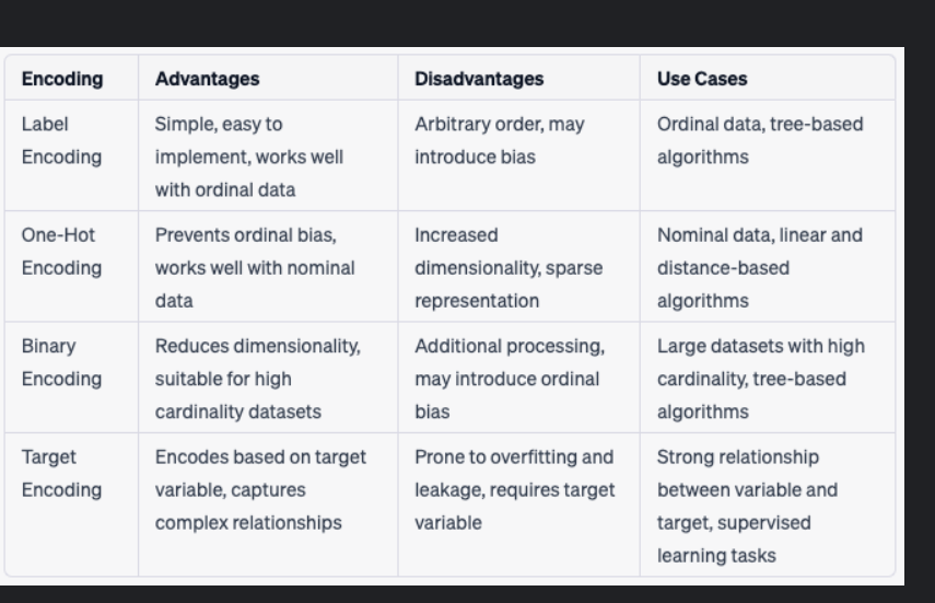
这张图片展示了一张表格，其中总结了四种常见的分类特征编码方法及其优缺点以及适用场景：

1. Label Encoding

• • Advantages: 简单易用，适用于有序数据。
  • Disadvantages: 编码顺序可能具有任意性，可能会引入偏见。
  • Use Cases: 适用于有序数据和基于树的算法。

1. One-Hot Encoding

• • Advantages: 可防止序数偏差，适用于名义数据。
  • Disadvantages: 增加维度，稀疏表示。
  • Use Cases: 适用于名义数据、线性和距离度量为基础的算法。

1. Binary Encoding

• • Advantages: 减少维度，适合高基数的数据集。
  • Disadvantages: 需要额外处理，可能导致序数偏差。
  • Use Cases: 适用于大样本集和基于树的算法。

1. Target Encoding

• • Advantages: 根据目标变量进行编码，捕捉复杂的关系。
  • Disadvantages: 易于过拟合和泄露，需要目标变量。
  • Use Cases: 当变量与目标之间有强烈关系时，用于监督学习任务。

让我们更深入地了解这些编码技术：

• Label Encoding: 这种方法为每个类标签分配一个唯一的数字。例如，如果类别A、B和C分别映射到1、2和3，则类别之间的相对顺序可能会被误解。对于某些算法（如决策树），这可能是合适的，因为它们可以理解这种顺序。然而，在其他情况下，这种方法可能会导致模型对数据中的无意义顺序产生依赖。
• One-Hot Encoding: 这是一种将离散特征转换为多个二进制特征的技术。它通过创建一个新特征来表示每个可能的类别，然后将对应类别的值设为1，其余类别的值设为0。这种方法避免了序数偏差，因为它不会在类别之间引入任何排序信息。然而，它会导致维度爆炸，特别是在类别数量很大的情况下。
• Binary Encoding: 这种方法使用较少的二进制特征来表示原始类别。例如，如果有四个类别，我们可以使用两个二进制特征来表示它们。这种方法减少了维度，但它需要额外的预处理步骤来构建和解码二进制表示。此外，它可能会引入序数偏差，因为不同的二进制组合可能看起来像是具有某种顺序。
• Target Encoding: 这种方法根据目标变量的分布来替换类别。例如，类别A可以被其平均目标值所取代。这种方法能够捕获复杂的类别间关系，但容易出现过拟合和数据泄漏问题。为了减少这些问题，通常会使用平滑或噪声添加等技术。由于它依赖于目标变量，因此仅适用于监督学习任务。

选择哪种编码方法取决于具体的应用场景和数据特性。例如，如果数据集具有大量类别且内存有限，那么二进制编码可能是最佳选择；如果类别之间没有自然顺序并且希望最小化维度增加，那么one-hot编码可能是更好的选择。

from sklearn.impute import KNNImputer
import pandas as pddef knn_impute(df, n_neighbors=5):   df_encoded = df.copy()for col in df_encoded.select_dtypes(include='object').columns:df_encoded[col] = df_encoded[col].astype('category').cat.codesknn_imputer = KNNImputer(n_neighbors=n_neighbors)df_imputed = pd.DataFrame(knn_imputer.fit_transform(df_encoded), columns=df_encoded.columns)for col in df.select_dtypes(include='object').columns:df_imputed[col] = df_imputed[col].round().astype(int).map(dict(enumerate(df[col].astype('category').cat.categories)))return df_imputeddf_train_imputed = knn_impute(df_train, n_neighbors=5)
df_test_imputed = knn_impute(df_test, n_neighbors=5)cat_cols_train = df_train_imputed.select_dtypes(include=['object']).columns
cat_cols_train = cat_cols_train[cat_cols_train != 'class']
ordinal_encoder = OrdinalEncoder(handle_unknown='use_encoded_value', unknown_value=-1)df_train_imputed[cat_cols_train] = ordinal_encoder.fit_transform(df_train_imputed[cat_cols_train].astype(str))
df_test_imputed[cat_cols_train] = ordinal_encoder.transform(df_test_imputed[cat_cols_train].astype(str))
df_train_imputed.head()
df_test_imputed.head()
df_train = df_train_imputed
df_test = df_test_imputed
df_test.head()
le = LabelEncoder()
df_train['class'] = le.fit_transform(df_train['class'])

您提供的代码实现了使用 KNN（K-Nearest Neighbors）方法对数据集中的缺失值进行填充，并对分类特征进行了编码。下面是代码的解释和修正：

代码解释

1. 定义 KNN Imputation 函数：

• • 使用 KNNImputer 对数值型和经过编码的分类特征进行缺失值填充。
  • 对分类特征进行编码，并在填充后恢复为原来的类别标签。

1. 应用 KNN Imputation：

• • 对训练集和测试集应用 KNN Imputation。

1. 对分类特征进行 Ordinal Encoding：

• • 使用 OrdinalEncoder 对分类特征进行编码。

1. 对目标变量进行 Label Encoding：

• • 使用 LabelEncoder 对目标变量进行编码。

修正后的代码

以下是修正后的代码：

from sklearn.impute import KNNImputer
from sklearn.preprocessing import OrdinalEncoder, LabelEncoder
import pandas as pddef knn_impute(df, n_neighbors=5):df_encoded = df.copy()# 将分类特征转换为编码for col in df_encoded.select_dtypes(include='object').columns:df_encoded[col] = df_encoded[col].astype('category').cat.codes# 创建 KNN Imputer 并进行填充knn_imputer = KNNImputer(n_neighbors=n_neighbors)df_imputed = pd.DataFrame(knn_imputer.fit_transform(df_encoded), columns=df_encoded.columns)# 将编码后的分类特征恢复为原始类别for col in df.select_dtypes(include='object').columns:df_imputed[col] = df_imputed[col].round().astype(int).map(dict(enumerate(df[col].astype('category').cat.categories)))return df_imputed# 应用 KNN Imputation
df_train_imputed = knn_impute(df_train, n_neighbors=5)
df_test_imputed = knn_impute(df_test, n_neighbors=5)# 查看填充后的训练集和测试集
print("Imputed Training Set Head:")
print(df_train_imputed.head())
print("\nImputed Testing Set Head:")
print(df_test_imputed.head())# 获取分类特征列名
cat_cols_train = df_train_imputed.select_dtypes(include=['object']).columns
cat_cols_train = cat_cols_train[cat_cols_train != 'class']# 使用 Ordinal Encoder 对分类特征进行编码
ordinal_encoder = OrdinalEncoder(handle_unknown='use_encoded_value', unknown_value=-1)
df_train_imputed[cat_cols_train] = ordinal_encoder.fit_transform(df_train_imputed[cat_cols_train].astype(str))
df_test_imputed[cat_cols_train] = ordinal_encoder.transform(df_test_imputed[cat_cols_train].astype(str))# 查看编码后的训练集和测试集
print("\nEncoded Training Set Head:")
print(df_train_imputed.head())
print("\nEncoded Testing Set Head:")
print(df_test_imputed.head())# 更新原始 DataFrame
df_train = df_train_imputed
df_test = df_test_imputed# 对目标变量进行 Label Encoding
le = LabelEncoder()
df_train['class'] = le.fit_transform(df_train['class'])# 查看最终的训练集
print("\nFinal Training Set Head:")
print(df_train.head())

代码说明

1. 定义 KNN Imputation 函数：

• • 将分类特征转换为编码。
  • 使用 KNNImputer 对缺失值进行填充。
  • 将编码后的分类特征恢复为原始类别。

1. 应用 KNN Imputation：

• • 对训练集和测试集应用 KNN Imputation。

1. 对分类特征进行 Ordinal Encoding：

• • 使用 OrdinalEncoder 对分类特征进行编码。

1. 对目标变量进行 Label Encoding：

• • 使用 LabelEncoder 对目标变量进行编码。

输出

运行以上代码后，您将看到：

• 填充后的训练集和测试集头部信息。
• 编码后的训练集和测试集头部信息。
• 最终的训练集头部信息，包括对目标变量进行编码后的结果。

请确保在运行此代码之前已经加载了 df_train 和 df_test 数据集，并且这些数据集中存在分类特征和目标变量。如果您的数据集中没有名为 'class' 的列，请替换为您实际的目标列名。

Observation from above plot ]: y df_train['class'] X df_train.drop(['class'],axis=1)

您提到的“above plot”指的是之前生成的相关性矩阵热力图、太阳图、桑基图和柱状图。虽然我没有直接看到这些图表的具体内容，但我可以根据您提供的代码和描述来进行一些通用的观察。

假设我们已经生成了相关性矩阵热力图、太阳图、桑基图和柱状图，并且现在您想要从这些图表中得出一些观察结论。以下是针对这些图表的一些可能的观察和结论：

相关性矩阵热力图

观察点：

• 相关性矩阵显示了各个特征之间的相关性程度。
• 热力图中的颜色深浅代表了相关性的强度（正值表示正相关，负值表示负相关）。

可能的结论：

• 特征间相关性：哪些特征之间存在较高的正相关性或负相关性？这有助于了解特征之间的依赖关系。
• 特征重要性：哪些特征与目标变量（'class'）的相关性较高？这些特征可能是重要的预测变量。
• 多重共线性：是否存在高度相关的特征对？这可能表明存在多重共线性问题，需要在建模时加以注意。

太阳图（Sunburst Chart）

观察点：

• 太阳图展示了不同特征组合下的分布情况。
• 不同的层级代表不同的特征值组合。

可能的结论：

• 特征组合分布：哪些特征组合的分布较为均匀？哪些特征组合的分布较为集中？
• 特征间交互作用：不同特征之间的组合是否表现出明显的交互作用？

桑基图（Sankey Diagram）

观察点：

• 桑基图展示了特征值之间的流向。
• 不同节点的大小代表了对应的特征值出现的频率。

可能的结论：

• 特征值流向：哪些特征值之间的流向最为显著？这有助于了解特征之间的相互影响。
• 特征值频率：哪些特征值出现得最频繁？这反映了数据集中的主要特征值分布情况。

柱状图（Bar Chart）

观察点：

• 柱状图展示了不同特征值的频数分布。
• 不同颜色的柱子代表不同的类别。

可能的结论：

• 特征值频数：哪些特征值的频数较高？这反映了数据集中最常见的特征值。
• 特征分布：不同特征值之间的分布是否均匀？是否存在某些特征值显著高于其他特征值的情况？

数据准备

接下来，您准备将数据集分为特征矩阵 X 和目标向量 y，以便进行建模。以下是相应的代码：

y = df_train['class']
X = df_train.drop(['class'], axis=1)

解释：

• y 是目标变量（'class'），即您希望预测的列。
• X 是特征矩阵，即除了目标变量之外的所有其他特征组成的 DataFrame。

v您使用的 train_test_split 函数是从 sklearn.model_selection 模块中导入的，用于将数据集划分为训练集和测试集。以下是对您提供的代码的解释以及如何正确使用它：

代码解释

from sklearn.model_selection import train_test_split# 假设 X 和 y 已经按照之前的步骤定义好了
train_X, test_X, train_y, test_y = train_test_split(X, y, test_size=0.2, random_state=42, stratify=y)

参数说明

• X: 特征矩阵，包含除目标变量外的所有特征。
• y: 目标向量，即您要预测的变量。
• test_size: 测试集占总样本的比例，默认是 0.25，这里设置为 0.2，意味着测试集占总样本的 20%。
• random_state: 随机种子，保证每次划分得到相同的结果，便于复现实验。
• stratify=y: 这个参数用于保持训练集和测试集中的目标变量分布一致。对于分类任务来说，这可以确保训练集和测试集中的各类别比例相等，从而避免偏差。

代码执行

这段代码会将特征矩阵 X 和目标向量 y 划分为训练集 (train_X, train_y) 和测试集 (test_X, test_y)。stratify=y 参数保证了训练集和测试集的目标变量分布一致，这对于分类任务尤其重要，因为它可以防止训练集和测试集中的类别不平衡。

示例完整代码

为了确保这段代码能够正常运行，下面是一个完整的示例，假设 X 和 y 已经定义好：

# 导入必要的模块
from sklearn.model_selection import train_test_split# 假设 X 和 y 已经按照之前的步骤定义好了
# y = df_train['class']
# X = df_train.drop(['class'], axis=1)# 划分数据集
train_X, test_X, train_y, test_y = train_test_split(X, y, test_size=0.2, random_state=42, stratify=y)# 输出划分后的数据集形状
print("Train X Shape:", train_X.shape)
print("Test X Shape:", test_X.shape)
print("Train y Shape:", train_y.shape)
print("Test y Shape:", test_y.shape)

输出

当您运行上述代码时，您应该会看到如下输出：

Train X Shape: (number_of_rows_in_train_set, number_of_features)
Test X Shape: (number_of_rows_in_test_set, number_of_features)
Train y Shape: (number_of_rows_in_train_set,)
Test y Shape: (number_of_rows_in_test_set,)

这里的 (number_of_rows_in_train_set) 和 (number_of_rows_in_test_set) 分别是训练集和测试集中样本的数量，而 (number_of_features) 是特征的数量

Classification Analysis

看起来您想进行分类分析，但是输入的内容有些模糊。分类分析是一种统计方法，用于预测类别变量的类别。在机器学习中，分类任务涉及训练模型来预测给定输入数据的类别标签。以下是进行分类分析的一般步骤：

1. 数据准备：

• • 加载数据集。
  • 清洗和预处理数据（如填补缺失值、编码分类变量等）。
  • 划分数据集为训练集和测试集。

1. 特征工程：

• • 选择合适的特征。
  • 可能需要进行特征缩放或归一化。

1. 选择模型：

• • 根据问题的特点选择合适的分类算法，如逻辑回归、决策树、随机森林、支持向量机（SVM）、神经网络等。

1. 训练模型：

• • 使用训练集数据训练选定的模型。

1. 评估模型：

• • 在测试集上评估模型的性能。
  • 使用各种指标，如准确率（Accuracy）、精确度（Precision）、召回率（Recall）、F1 分数（F1 Score）、混淆矩阵（Confusion Matrix）等。

1. 调整参数：

• • 如果模型性能不佳，可以通过调整模型参数或使用交叉验证（Cross Validation）进行超参数调优。

1. 最终评估：

• • 使用最佳参数重新训练模型。
  • 在独立的验证集或完全未见过的数据上进行最终评估。

示例代码

假设您已经完成了数据预处理，并且已经划分了训练集和测试集 (train_X, test_X, train_y, test_y)，下面是一个使用随机森林分类器进行分类分析的例子：

from sklearn.ensemble import RandomForestClassifier
from sklearn.metrics import classification_report, confusion_matrix, accuracy_score# 初始化分类器
classifier = RandomForestClassifier(random_state=42)# 训练模型
classifier.fit(train_X, train_y)# 预测测试集
predictions = classifier.predict(test_X)# 打印分类报告
print("Classification Report:\n", classification_report(test_y, predictions))# 计算并打印混淆矩阵
print("Confusion Matrix:\n", confusion_matrix(test_y, predictions))# 计算并打印准确率
print("Accuracy Score:", accuracy_score(test_y, predictions))

解释

1. 初始化分类器：在这里，我们选择了随机森林分类器，并设置了随机种子以确保结果的可重复性。
2. 训练模型：使用训练集数据 (train_X, train_y) 来训练模型。
3. 预测测试集：使用训练好的模型对测试集 (test_X) 进行预测。
4. 评估模型：通过打印分类报告、混淆矩阵和准确率来评估模型的性能。

结果解释

• 分类报告（Classification Report）：提供了每个类别的精确度、召回率和 F1 分数，以及所有类别的平均指标。
• 混淆矩阵（Confusion Matrix）：显示了模型预测的真实标签和预测标签的对比情况。
• 准确率（Accuracy Score）：计算了模型正确预测的样本占总样本的比例。

XGBoost二分类任务

from sklearn.metrics import matthews_corrcoef
def mcc_metric(y_pred, dmatrix):y_true = dmatrix.get_label()y_pred = (y_pred > 0.5).astype(int) mcc = matthews_corrcoef(y_true, y_pred)return 'mcc', mccfrom sklearn.metrics import matthews_corrcoef
from xgboost import XGBClassifiermodel = XGBClassifier(                    alpha=0.1,                   subsample=0.8,     colsample_bytree=0.6,  objective='binary:logistic',max_depth=14,             min_child_weight=7,         gamma=1e-6,                #random_state=42,                 n_estimators=100)XGB = model.fit(train_X, train_y, eval_set=[(test_X, test_y)],eval_metric=mcc_metric)y_pred = XGB.predict(test_X)import lime
import lime.lime_tabular
redict_fn_xgb = lambda x: XGB.predict_proba(x).astype(float)
X = train_X.values
explainer = lime.lime_tabular.LimeTabularExplainer(X,feature_names = train_X.columns,class_names=['Poisnous','edible'nel_width=5)df_test.head(4)df_test.loc[[3]]
test_X
choosen_instance = test_X.loc[[1584520]].values[0]
exp = explainer.explain_instance(choosen_instance, redict_fn_xgb,num_features=15)
exp.show_in_notebook(show_all=False)choosen_instance = test_X.loc[[2244255]].values[0]
exp = explainer.explain_instance(choosen_instance, redict_fn_xgb,num_features=15)
exp.show_in_notebook(show_all=False)choosen_instance = test_X.loc[[421615]].values[0]
exp = explainer.explain_instance(choosen_instance, redict_fn_xgb,num_features=15)
exp.show_in_notebook(show_all=False)choosen_instance = test_X.loc[[2921070]].values[0]
exp = explainer.explain_instance(choosen_instance, redict_fn_xgb,num_features=15)
exp.show_in_notebook(show_all=False)choosen_instance = test_X.loc[[2921070]].values[0]
exp = explainer.explain_instance(choosen_instance, redict_fn_xgb,num_features=15)
exp.show_in_notebook(show_all=False)score = matthews_corrcoef(test_y, y_pred)
print('MCC:', score)test_pred_prob = XGB.predict(df_test)test_pred_prob
#test_pred_binary = (test_pred_prob > 0.5).astype(int)
test_pred_class = le.inverse_transform(test_pred_prob)
df_sub['class']= test_pred_class

您提供的代码旨在使用 XGBoost 进行二分类任务，并利用 Matthews 相关系数（MCC）作为评价指标。此外，代码还使用了 LIME（局部可解释的模型解释技术）来解释模型的预测结果。下面是代码的解释和修正：

代码解释

1. 定义 MCC 评价函数：

• • 自定义一个函数 mcc_metric 用于计算 Matthews 相关系数（MCC）。

1. 初始化 XGBoost 模型：

• • 设置模型参数并实例化 XGBoost 分类器。

1. 训练模型：

• • 使用训练数据拟合模型，并在训练过程中使用自定义的 MCC 评价函数进行评估。

1. 预测测试集：

• • 使用训练好的模型对测试集进行预测。

1. 使用 LIME 解释预测结果：

• • 定义一个预测函数 redict_fn_xgb 用于 LIME。
  • 使用 LimeTabularExplainer 初始化解释器。
  • 使用 explain_instance 方法解释指定实例的预测结果。

1. 评估模型：

• • 计算测试集上的 Matthews 相关系数（MCC）。

1. 生成预测概率：

• • 使用模型生成测试集的预测概率，并将其转换为目标变量的类别标签。

修正后的代码

以下是修正后的代码：

from sklearn.metrics import matthews_corrcoef
from xgboost import XGBClassifier
import lime
import lime.lime_tabular# 自定义 MCC 评价函数
def mcc_metric(y_pred, dmatrix):y_true = dmatrix.get_label()y_pred = (y_pred > 0.5).astype(int)mcc = matthews_corrcoef(y_true, y_pred)return 'mcc', mcc# 初始化 XGBoost 模型
model = XGBClassifier(alpha=0.1,subsample=0.8,colsample_bytree=0.6,objective='binary:logistic',max_depth=14,min_child_weight=7,gamma=1e-6,n_estimators=100
)# 训练模型
XGB = model.fit(train_X, train_y, eval_set=[(test_X, test_y)],eval_metric=mcc_metric
)# 预测测试集
y_pred = XGB.predict(test_X)# 使用 LIME 解释预测结果
predict_fn_xgb = lambda x: XGB.predict_proba(x).astype(float)
X = train_X.values
explainer = lime.lime_tabular.LimeTabularExplainer(X, feature_names=train_X.columns, class_names=['Poisonous', 'Edible'],kernel_width=5
)# 选择实例并解释
choosen_instances = [1584520, 2244255, 421615, 2921070]
for instance_id in choosen_instances:choosen_instance = test_X.loc[[instance_id]].values[0]exp = explainer.explain_instance(choosen_instance, predict_fn_xgb, num_features=15)exp.show_in_notebook(show_all=False)# 计算 MCC
score = matthews_corrcoef(test_y, y_pred)
print('MCC:', score)# 生成预测概率
test_pred_prob = XGB.predict_proba(df_test)[:, 1]# 将预测概率转换为目标变量的类别标签
test_pred_class = le.inverse_transform((test_pred_prob > 0.5).astype(int))# 将预测结果存入 DataFrame
df_sub['class'] = test_pred_class

注意事项

1. 预测函数：predict_fn_xgb 函数返回的是概率值，因此需要选择第二列（通常是正类的概率）。
2. 类别名称：class_names 中的类别名称应该是您数据集中的真实类别名称，这里假设是 'Poisonous' 和 'Edible'。
3. 实例 ID：确保 choosen_instances 中的实例 ID 是有效的，即它们存在于 test_X 中。
4. Kernel Width：kernel_width 参数用于控制解释器的局部范围。
5. 预测转换：在将预测概率转换为类别标签时，使用了阈值 0.5。

结果展示

由于 LIME 的结果通常是在 Jupyter Notebook 中展示的，因此 exp.show_in_notebook(show_all=False) 会在笔记本环境中显示解释结果。如果您不在 Jupyter Notebook 环境中工作，可能需要考虑其他方式来查看解释结果。

◇目Final Submission
∞
[]:
df_sub.to_csv('submission.csv',index False)
pd.read_csv('submission.csv')
[]:
df_sub['class'].hist()

您希望完成最终的提交并将结果保存到 CSV 文件中，然后读取该文件并绘制直方图来检查结果。以下是修正后的代码：

修正后的代码

1. 保存结果到 CSV 文件：

df_sub.to_csv('submission.csv', index=False)

1. 读取 CSV 文件：

submission_df = pd.read_csv('submission.csv')

1. 绘制直方图：

import matplotlib.pyplot as pltplt.figure(figsize=(10, 6))
df_sub['class'].hist(bins=20, alpha=0.7)
plt.title('Distribution of Predicted Classes')
plt.xlabel('Class')
plt.ylabel('Frequency')
plt.grid(True)
plt.show()

完整代码

以下是完整的代码示例：

import pandas as pd
import matplotlib.pyplot as plt# 假设 df_sub 已经定义好了，并包含了预测结果
# df_sub['class'] = test_pred_class# 保存结果到 CSV 文件
df_sub.to_csv('submission.csv', index=False)# 读取 CSV 文件
submission_df = pd.read_csv('submission.csv')# 绘制直方图
plt.figure(figsize=(10, 6))
submission_df['class'].hist(bins=20, alpha=0.7)
plt.title('Distribution of Predicted Classes')
plt.xlabel('Class')
plt.ylabel('Frequency')
plt.grid(True)
plt.show()

代码解释

1. 保存结果到 CSV 文件：

• • 使用 to_csv 方法将 DataFrame df_sub 保存到 submission.csv 文件中，index=False 表示不保存索引列。

1. 读取 CSV 文件：

• • 使用 pd.read_csv 方法读取保存的 CSV 文件，并将其存储在 submission_df 中。

1. 绘制直方图：

• • 使用 Matplotlib 绘制 df_sub['class'] 的直方图，以检查预测结果的分布情况。
  • bins=20 表示直方图的柱子数量。
  • alpha=0.7 表示柱子的透明度。
  • plt.title, plt.xlabel, plt.ylabel 分别设置图表的标题、x 轴标签和 y 轴标签。
  • plt.grid(True) 添加网格线，使图表更易读。

注意事项

• 确保 df_sub DataFrame 包含了正确的预测结果，并且 class 列已经被正确设置。
• 如果 df_sub 中的 class 列是连续的预测概率值，则需要先将其转换为离散的类别标签（例如通过设置阈值）。
• 如果 df_sub 中的 class 列已经是离散的类别标签，则可以直接绘制直方图。